Sometimes we face problems that look very simple at first sight but reveal to be complicated to code. Network clustering is one of those: with patience, anyone can manually pool all the nodes of a network into connex sets by "manually" following all the links one by one. But when it comes to write a script that reproduces this simple strategy, finding an elegant and efficient code is far from obvious. Actually the problem is related to labelling connected-components and anyone that has already tried to code this basic computer vision task knows what I'm talking of.
In this post I review three different methods to extract clusters from an adjacency matrix. A simple benchmark compares their performance and show that the reverse Cuthill-McKee algorithm improves execution time by a factor 30 as compared to brute force.
As a start, we need nodes. For convenience I will use here an hexagonal mesh but any other mesh (e.g. square or random) would fit. Here is the Matlab mesh generation code:
% --- Parameters

a = 10;          % Mesh width
p = 0.25;        % Link probability

% --- Hexagonal mesh

[X, Y] = meshgrid(1:a, 1:a);
for i = 2:2:a
	X(i,:) = X(i,:) + 1/2;
end
Y = Y*sqrt(3)/2;
x = X(:);
y = Y(:);
Then let's generate a random network on this mesh. To this aim, we can determine all the possible neighboring links (via a Delaunay triangulation) and keep only a certain amount of these links, chosen at random. For the rest of this post I will place myself below the percolation threshold by keeping a fraction of $p=0.25$ links:
% --- Random network generation

% Get delaunay triangulation
T = delaunay(x, y);

% Get a list of all links
tmp = [T(:,1) T(:,2) ; T(:,1) T(:,3) ; T(:,2) T(:,3)];

% Filter out duplicates
links = unique([min(tmp(:,1), tmp(:,2)), max(tmp(:,1), tmp(:,2))], 'rows');

% Filter with probability p to get the random network
L = links(rand(size(links,1),1)<=p, :);

% Get sparse adjacency matrix
A = sparse(L(:,1), L(:,2), ones(size(L,1),1), a^2, a^2);
The main output of this piece of code is the adjacency matrix $A$. It is an array that contains all the information about the network connectivity. Note that I use sparse matrices by default, to push back the problems related to the large size limit.
A note on symmetry
Though adjacency matrices do not have to be symmetrical, making clusters require that "connections" are reciprocal. Otherwise the algorithm's output might be different between executions, depending on the algorithm or the seed. To prevent from this, the adjacency matrices are automatically symmetrized in all proposed methods. Thus, the adjacency matrix that is this passed to the
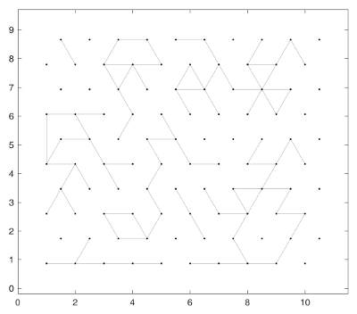
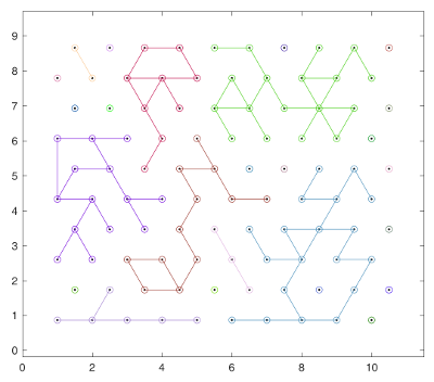
Here is the generated network and the result of the clusterization (any of the three following methods would give the same result):
Method 1: Brute force
As usual, brute force is the first idea that come to one's mind. A simple idea is to start from a seed and iteratively store its connected nodes, while removing them from the list of unexplored nodes. Being brutal doesn't prevent to be smart though, and the functions
function C = adj2cluster_bf(A)

% Symmetrize adjacency matrix
S = A + A';

% Initialization
C = {};
I = 1:size(S,1);

% The main loop
while ~isempty(I)
    C{end+1} = [];
    J = I(1);
    while ~isempty(J)
        C{end}(end+1) = J(1);
        J = setdiff(union(J, find(S(J(1),:))), C{end});
    end
    I = setdiff(I, C{end});
end
Method 2: Powering the matrix
To fasten the execution time, it would be beneficial to transform the matrix to work with in a form that is easier to process. For instance, if all nodes were connected to all other node of the cluster, it would be fairly easier. To this aims, one can use the fact that the powers of the adjacency matrix give the number of walks between any two vertices ; by summing all the powers of the adjacency matrix $R_q = A + A^2 + ... + A^q$ up to the point where no more $R_q(i,j)$ term becomes non-zero, one gets a network with fully-connected clusters.
Here is a possible implementation:
function C = adj2cluster_mp(A)

% Symmetrize adjacency matrix
S = A + A';

% Create fully-connected subnetworks
P = S;
R = S;
i = 1;
while true
    P = P*S;
    T = R + P;
    if any(boolean(T(:))~=boolean(R(:)))
        R = T;
    else
        break
    end
end

% Extract the clusters
C = {};
I = 1:size(A,1);
while ~isempty(I)
    J = [I(1) find(R(I(1),:))];
    C{end+1} = J;
    I = setdiff(I,J);
end
As you will see in the benchmark section, this method is faster than brute force. But wait a moment, there is a third method.
Method 3: Using the reverse Cuthill-McKee algorithm
Another idea is to reorder the adjacency matrix in a diagonal-by-blocks form. Many algorithms can do that, but the reverse Cuthill-McKee algorithm works very well in our case since the blocks are directly the clusters. Icing on the cake: it is already implemented with the built-in
Here is the code:
function C = adj2cluster(A)

% Symmetrize adjacency matrix
S = A + A';

% Reverse Cuthill-McKee ordering
r = fliplr(symrcm(S));

% Get the clusters
C = {r(1)};
for i = 2:numel(r)
    if any(S(C{end}, r(i)))
        C{end}(end+1) = r(i);
    else
        C{end+1} = r(i);
    end
end
Pretty simple, isn't it ?
Benchmark and discussion
All three methods give the same result, so to compare them the execution time is a critical measurement. I have generated random networks of various sizes up to more than 10,000 points with a connectivity fraction of $p=0.25$ and applied the three clusterization methods to these networks. I obtain the following graph:
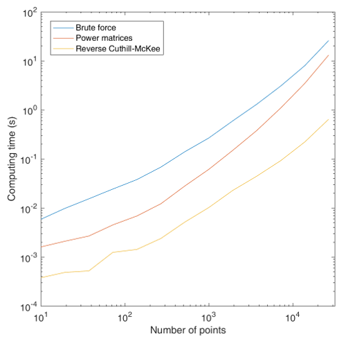
As you can see, the third method is much faster, with an average 5-fold gain with respect to the "Power matrices" method and an average 30-fold gain as compared to brute force. But it may not be completely optimized, and I think one could still find a faster way. So this is an open challenge: can you find a more efficient implementation?
Downloads
The code of the third method (the fastest) can be downloaded on Matlab's File Exchange.
Have fun !
Comments
Thanks for your kind message! Glad it could help. Best regards
Dear Raphaël, Your explanations are clear, simple and straight to the point. The text you shared here, along with the kindly provided code is very useful. I truly enjoyed reading it. Thank you!